Fine Control the Evolution Process¶

Oftentimes, we may want to adjust reproduction behaviors while evolution progresses. For example, to explore more at the beginning, and to exploit more at the later stage of the search. This notebook illustrates how to fine control such behaviors during the evolution process, through PyGlove’s symbolic scalar system. In fact, almost all built-in operations provided by PyGlove support hyperparameters controlled by such scalars. Before we get into a rich library of scalars, let’s start with a simple case which decays the mutation probability as the search progresses.

!pip install pyglove

import pyglove as pg

Getting Started: Mutation with decaying probability¶

First, let’s mutate a DNA with the same probability (0.9) along the whole evolution process:

dna_spec = pg.dna_spec(pg.oneof(range(10)))
dna = dna_spec.first_dna()
print(dna)

DNA(0)

# Mutate a DNA with prability 0.9.
op = pg.evolution.mutators.Uniform(seed=1).with_prob(0.9)
for _ in range(10):
  dna = op([dna])[0]
  print(dna)

DNA(9)
DNA(4)
DNA(7)
DNA(7)
DNA(3)
DNA(7)
DNA(6)
DNA(9)
DNA(7)
DNA(3)

Assume we will run the search with 20 generations, can we gradually reduce the mutation probability from 1.0 to 0.0? Here is the answer:

op = pg.evolution.mutators.Uniform(seed=1).with_prob(
    pg.scalars.linear(20, 1.0, 0.0), seed=1)

dna = dna_spec.first_dna()
for i in range(20):
  dna = op([dna], step=i)[0]
  print(dna)

DNA(9)
DNA(4)
DNA(7)
DNA(7)
DNA(3)
DNA(7)
DNA(6)
DNA(6)
DNA(9)
DNA(7)
DNA(7)
DNA(3)
DNA(3)
DNA(5)
DNA(5)
DNA(5)
DNA(5)
DNA(5)
DNA(5)
DNA(0)

PyGlove’s Symbolic Scalar System¶

Before we introduce PyGlove’s symbolic scalar system, let’s take a look at the mechanism for supporting evolution behavior scheduling.

Step-based Hyperparameters¶

As introduced in Evolutionary Algorithm, evolutionary operations in PyGlove can take a step argument when processing the input. This means, if an operation is controlled by a hyperparameter (e.g. probability), the hyperparameter can be a function of step. Therefore, we can pass a function to pg.evolution.selectors.Top as the value for n:

dna_list = [
  pg.evolution.set_fitness(pg.DNA(i), i)
  for i in range(10)
]

op = pg.evolution.selectors.Top(lambda x: x)

print(op(dna_list, step=0))
print(op(dna_list, step=1))
print(op(dna_list, step=2))

[]
[DNA(9)]
[DNA(9), DNA(8)]

Symbolic Scalars: Reusable & compositional functions for hyperparameter scheduling¶

It’s natural to think about how to make the functions for producing hyperparameters reusable, preferrably compositional. PyGlove introduces pg.scalars sub-module for such purpose. A scalar is a callable symbolic object that produces a value based on a step, defined as:

class Scalar(pg.Object):
  def __call__(self, step: int) -> Any

For example, pg.scalars.STEP is a singleton Scalar subclass which returns the current step. Scalar overloads operators such as __add__, __sub__, so the scalar objects can be combined as regular math expressions. For example:

h = (pg.scalars.Constant(2) 
     + pg.scalars.linear(total_steps=10, start=0, end=10))
print(h)
print(h(10))

Addition(
  x = Constant(
    value = 2
  ),
  y = Addition(
    x = 0,
    y = Multiplication(
      x = _Step(),
      y = 1.0
    )
  )
)
12.0

In order for an operation to use a scalar as hyperparameter, all it needs is to:

define its hyperparameter using pg.scalars.scalar_spec.
get the scalar value at a given step using pg.scalars.scalar_value.

For example, pg.evolution.selectors.Top defines and consumes its argument n in the following way:

@pg.mebmers([
  ('n', pg.scalars.scalar_spec(pg.typing.Int(min_value=0)))
])
class Top(pg.evolution.Selector)
  def select(self, inputs, step):
    n = pg.scalars.scalar_value(self.n, step)
    ...

A Catalog of Built-in Scalars¶

PyGlove provides a rich set of built-in scalars for addressing most common scheduling needs, including basic math operations, random number generators and common decay functions. It also provides a StepWise schedule to work with pg.evolution.Conditional operator to generate complex evolution processes.

import matplotlib.pyplot as plt

def render_scalar(scalar, steps=100):
  ys = [scalar(step=i) for i in range(1, steps + 1)]
  plt.plot(ys)

Basic Scalars¶

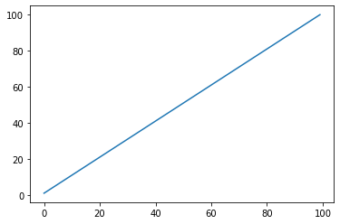
STEP: Returns current step¶

s = pg.scalars.STEP
render_scalar(s)

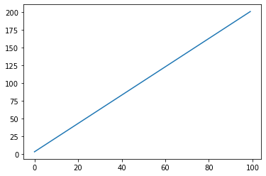
../../../_images/d86bfd7a703cd6271a1869d2049e46bdbc725dfc9617c6898f41bcd8bd2eded6.png

Lambda: Converts a function into a scalar¶

s = pg.scalars.Lambda(lambda step: step * 2) + 1
render_scalar(s)

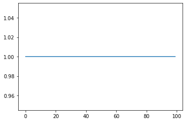
../../../_images/592ce51390bed98533c8dc8ff939e41dfe76d08364fd5ac11042b2fca124c1df.png

Constant: Returns a constant as scalar¶

s = pg.scalars.Constant(1)
render_scalar(s)

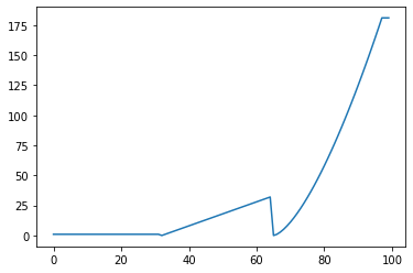
../../../_images/a73433b21ce53be0a6689ab9b9fdc5de876dc9bd7bfe617af93b974e6e4ce78f.png

StepWise: Step-wise scalar¶

s = pg.scalars.StepWise([
    (0.2, 1),
    # pg.scalars.STEP means step within current phase
    # in the context of step-wise scalar.
    (0.2, pg.scalars.STEP),
    (0.2, pg.scalars.STEP ** 1.5),
], total_steps=100)
render_scalar(s)

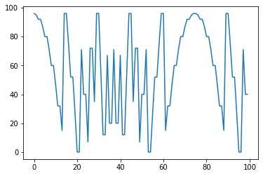
../../../_images/145e3d98388497775ea2c78774a432239080461d29f6679a35abd578a0fe1a68.png

Math Expressions¶

Common Math Operations¶

s = (-(pg.scalars.STEP * 2 // 3) ** 2 - 5 + 1) % 100
render_scalar(s)

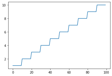
../../../_images/e7484a0fe6716a4d20aeaddc2d856e927c121130155526838aadd16ad0a05e4a.png

Ceiling: Returns ceil(x)¶

s = pg.scalars.Ceiling(pg.scalars.STEP / 10)
render_scalar(s)

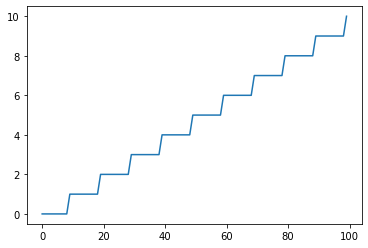
../../../_images/1ba17759ea459b9c70fe24965f58ef7b1158ca31e7f000242534b4911a0ddf7b.png

Floor: Returns floor(x)¶

s = pg.scalars.Floor(pg.scalars.STEP / 10)
render_scalar(s)

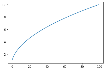
../../../_images/a6b60abccbe7e9347a659be1637f9ee6dfbf310b6d65a4b081a7019e8ff9a48c.png

SquareRoot/sqrt: Returns sqrt(x)¶

s = pg.scalars.sqrt(pg.scalars.STEP)
render_scalar(s)

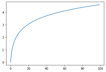
../../../_images/74823c6c145dcba4f6f7076e4a3fb1189b1354c72c1f60ef19887f0b06de444d.png

Log/log: Returns log(x)¶

s = pg.scalars.log(pg.scalars.STEP)
render_scalar(s)

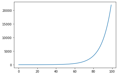
../../../_images/b32a7931f311d4fe602bcc4f1ae16db97f96b38772ef581bea59a3445494cf90.png

Exp/exp: Returns exp(x)¶

s = pg.scalars.exp(pg.scalars.STEP / 10)
render_scalar(s)

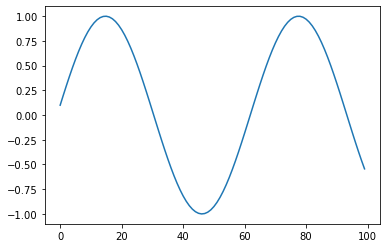
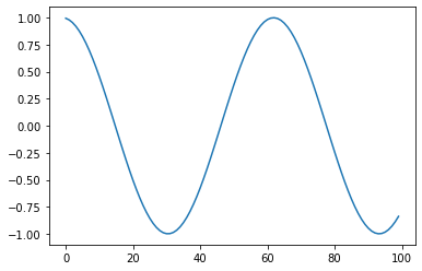
../../../_images/016562d2757fbf6b88e89c70083a02326adc04774932a185e9bcf239970a7e76.png

Sine/sin: Returns sine(x)¶

s = pg.scalars.sin(pg.scalars.STEP / 10)
render_scalar(s)

../../../_images/b66a9515bc54cce8fb31b2384169d2ae83da4c993832582bf20ea36eb05348b3.png

Cosine/cos: Returns Cosine(x)¶

s = pg.scalars.cos(pg.scalars.STEP / 10)
render_scalar(s)

../../../_images/2db00cad6e78eb3c121adbd3a4fd37cf2e102205080525953def04d8acfcaac7.png

Common Decay Helpers¶

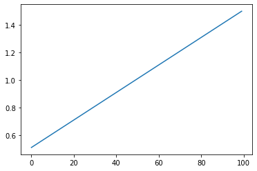
Linear: Linear scaling based on STEPS¶

s = pg.scalars.linear(100, 0.5, 1.5)
render_scalar(s)

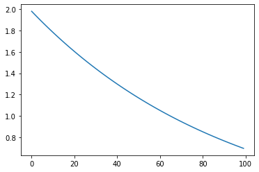
../../../_images/1dcec5fa3dfbb092d3f0a61e669bad11be4e6faeccf971608252e302c0d3e1c6.png

Exponential Decay: Exponential scaling based on STEPS¶

s = pg.scalars.exponential_decay(
    decay_rate=0.9, decay_interval=10, start=2.0, staircase=False)
render_scalar(s)

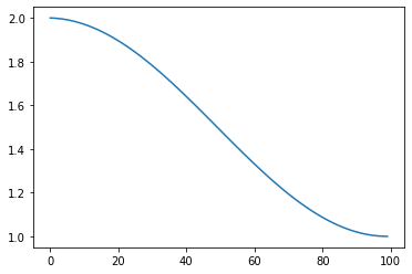
../../../_images/d3fccbecdf049f427fd65abfae2ed843ff01e40d1bf3786ebbff5d4c65ad2fec.png

Cosine Decay: Cosine decay based on STEPS¶

s = pg.scalars.cosine_decay(
    total_steps=100, start=2.0, end=1.0)
render_scalar(s)

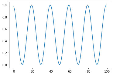
../../../_images/b3e40423451fdbdc1eefb7ed7d8e7f687c8b096acad7709d48ca9001613cce64.png

Cyclic: Cyclic scaling based on STEPS¶

s = pg.scalars.cyclic(cycle=20)
render_scalar(s)

../../../_images/dfe8d80208a759f500af7c1c016c1cfa4b5f0dba2cf53daed80546a163e52413.png

Random Numbers¶

def render_distribution(scalar, steps=1000):
  plt.hist([scalar(step=i) for i in range(1, steps + 1)])

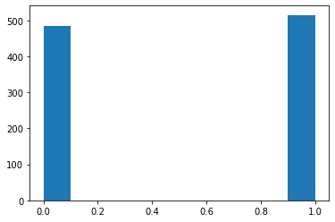
Uniform: Returns a random number in uniform distribution.¶

# Returns a random int from a range.
s = pg.scalars.Uniform(0, 1, seed=1)
render_distribution(s)

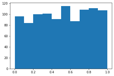
../../../_images/be4648c50638991913a924be535f28d5c20e125cd68bb479d1556f9396398f55.png

# Returns a random float from a range.
s = pg.scalars.Uniform(0.0, 1.0, seed=1)
render_distribution(s)

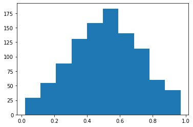
../../../_images/9ccecc7c5407edfa295113031d0ee34b16d7ab7d4d0bde4001aa1d167c99863a.png

Triangular: Returns a random float number in triangular distribution.¶

s = pg.scalars.Triangular(0.0, 1.0, seed=1)
render_distribution(s)

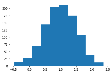
../../../_images/4fec15c43b4b004765e02758927554c35626f9d037029446207b069c53b0575e.png

Gaussian: Returns a random float number in gaussian distribution.¶

s = pg.scalars.Gaussian(mean=1.0, std=0.5, seed=1)
render_distribution(s)

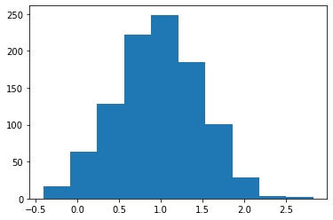
../../../_images/578a10bc1b201221ccec5325a9e56b73d37cd2e555e80441221e3a56909f9d1b.png

Normal: Returns a random float number in normal distribution.¶

s = pg.scalars.Normal(mean=1.0, std=0.5, seed=1)
render_distribution(s)

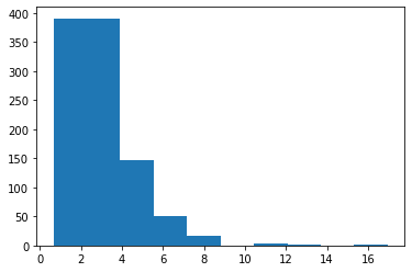
../../../_images/82ff7e8f2d3b2389b68f99394307fd4dd6223b5ad5206cd1611f413bb0166294.png

LogNormal: Returns a random float number in log normal distribution.¶

s = pg.scalars.LogNormal(mean=1.0, std=0.5, seed=1)
render_distribution(s)

../../../_images/99e65d2d647581050159c95110123f82155e3d8c5505dc2a8d0be73c404d3f57.png