Symbolic Machine Learning
![]()
Machine learning (ML) is sensitive to neural architectures and hyperparameters, making their representation critical to the design of an ML system. ML practitioners rely on these representations to conduct experiments and deploy models in production.
In a traditional ML system, ML components are built to serve the system’s purpose, with a separate configuration system used to adjust their hyperparameters. This requires developers and users to maintain a mapping between the components and their configurations, ensuring that they remain consistent. PyGlove offers an alternative approach by using symbolic classes to develop ML components. Symbolic objects are a natural and mutable representation of these components, eliminating the need for a separate configuration system. As a result, symbolic ML systems are simpler and more user-friendly. In this Colab, we provide an example of a symbolic ML pipeline that can support the entire experimentation life-cycle with ease and power.
!pip install pyglove
An Overview of a Symbolic ML Experiment
In PyGlove, an ML pipeline (or experiment) can be represented as a symbolic object - an object that can be manipulated safely after their creation based on their construction signatures. The root object is the whole experiment, whose sub-nodes are symbolic objects of ML components that specify the details of the experiment.
All ML components (including the Experiment class) are symbolic, meaning that they can be safely manipulated after creation. With PyGlove, users can create a symbolic class by extending pg.Object or symbolizing a regular class via pg.symbolize. The code below shows the definition of Experiment class, and lower-level ML components symbolized from functions or Keras classes.
import tensorflow as tf
import pyglove as pg

@pg.members([
  ('model', pg.typing.Object(tf.keras.Model),
   'Model used for both training and evaluation.'),
  ('training', pg.typing.Dict([
    ('input', pg.typing.Callable(),
     'A callable that returns a tuple of (features, labels) for training.'),
    ('batch_size', pg.typing.Int(min_value=1),
     'Training batch size.'),
    ('num_epochs', pg.typing.Int(min_value=1),
     'Number of epochs for training.'),
    ('loss', pg.typing.Object(tf.keras.losses.Loss),
     'Loss used for optimization.'),
    ('optimizer', pg.typing.Object(tf.keras.optimizers.Optimizer),
     'Optimizer for minimizing the loss.'),
  ])),
  ('evaluation', pg.typing.Dict([
    ('input', pg.typing.Callable(),
     'A callable that returns a tuple of (feature, labels) for evaluation.'),
    ('batch_size', pg.typing.Int(min_value=1),
     'Evaluation batch size.'),
    ('metric', pg.typing.Object(tf.keras.metrics.Metric),
     'Evaluation metrics.')
  ]))
])
class Experiment(pg.Object):

  def run(self):
    self.model.compile(
        optimizer=self.training.optimizer,
        loss=self.training.loss,
        metrics=[self.evaluation.metric])
    x_train, y_train = self.training.input()
    self.model.fit(x_train, y_train, epochs=self.training.num_epochs)

    x_test, y_test = self.evaluation.input()
    _, test_metric = self.model.evaluate(x_test, y_test)
    return test_metric


# Create an experiment instance.
@pg.symbolize
def mnist(training):
  (x_train, y_train),(x_test, y_test) = tf.keras.datasets.mnist.load_data()
  x_train, x_test = x_train / 255.0, x_test / 255.0
  if training:
    x_train /= 255.0
    return x_train, y_train
  else:
    x_test /= 255.0
    return x_test, y_test

# Symbolize regular Keras classes to make them serializable.
Sequential = pg.symbolize(tf.keras.Sequential)
Flatten = pg.symbolize(tf.keras.layers.Flatten)
Dense = pg.symbolize(tf.keras.layers.Dense)
Dropout = pg.symbolize(tf.keras.layers.Dropout)
Adam = pg.symbolize(tf.keras.optimizers.Adam)
SparseCategoricalCrossentropy = pg.symbolize(
    tf.keras.losses.SparseCategoricalCrossentropy)
SparseCategoricalAccuracy = pg.symbolize(
    tf.keras.metrics.SparseCategoricalAccuracy)
With symbolic classes, an experiment can be expressed as an Experiment. And we can run the experiment by calling its run method, and save it for reproduction later.
# Create an instance of Experiment via composition.
exp1 = Experiment(
  model=Sequential(layers=[
     Flatten(input_shape=(28, 28)),
     Dense(1024, activation='relu'),
     Dropout(0.2),
     Dense(10, activation='softmax')
  ]),
  training=pg.Dict(
      input=mnist(training=True),
      batch_size=32,
      num_epochs=2,
      loss=SparseCategoricalCrossentropy(),
      optimizer=Adam(),
  ),
  evaluation=pg.Dict(
      input=mnist(training=False),
      batch_size=32,
      metric=SparseCategoricalAccuracy()
  ))

# Run and save experiment.
exp1.run()
exp1.save('exp1.json')
Downloading data from https://storage.googleapis.com/tensorflow/tf-keras-datasets/mnist.npz
11490434/11490434 [==============================] - 0s 0us/step
Epoch 1/2
1875/1875 [==============================] - 9s 4ms/step - loss: 0.7588 - sparse_categorical_accuracy: 0.8040
Epoch 2/2
1875/1875 [==============================] - 6s 3ms/step - loss: 0.3478 - sparse_categorical_accuracy: 0.9005
313/313 [==============================] - 1s 2ms/step - loss: 0.3042 - sparse_categorical_accuracy: 0.9105
Life-cycle of a Symbolic ML Experiment
Most advancements in machine learning are based on iterating existing experiments. The life-cycle for experimenting a new idea can be described in 4 phases:

Reproduction
Reproducing an existing experiment is simply clone the existing experiment object, or load if from a saved JSON file.
experiment = exp1.clone(deep=True)
assert pg.eq(experiment, exp1)

experiment = pg.load('exp1.json')
assert pg.eq(experiment, exp1)

experiment.run()
Epoch 1/2
1875/1875 [==============================] - 6s 3ms/step - loss: 0.7663 - sparse_categorical_accuracy: 0.8054
Epoch 2/2
1875/1875 [==============================] - 7s 4ms/step - loss: 0.3503 - sparse_categorical_accuracy: 0.9003
313/313 [==============================] - 1s 3ms/step - loss: 0.3026 - sparse_categorical_accuracy: 0.9126
0.9125999808311462
Modification
To iterate an idea, an existing ML experiment needs to be modified into new ones. With PyGlove, a symbolic object can be manipluated into another object without modifying existing code. This gives the maximum flexibility to accomondate unanticpated changes when new ideas pop up.
@pg.symbolize
class NewModel(tf.keras.Model):

  def __init__(self, activation):
    super().__init__()
    self._dense1 = Dense(1024, activation=activation)
    self._dense2 = Dense(10, activation='softmax')

  def call(self, inputs):
    x = Flatten()(inputs)
    x = self._dense1(x)
    x = Dropout(0.2)(x)
    x = self._dense2(x)
    return x

ReLU = pg.symbolize(tf.keras.layers.ReLU)
RMSProp = pg.symbolize(tf.keras.optimizers.RMSprop)

experiment.rebind({
  'model': NewModel(activation=ReLU()),
  'training.batch_size': 256,
  'training.optimizer': RMSProp(0.01)
})
print(experiment)
experiment.run()
Experiment(
  model = NewModel(
    activation = ReLU(
      max_value = None,
      negative_slope = 0.0,
      threshold = 0.0
    )
  ),
  training = {
    input = mnist(
      training = True
    ),
    batch_size = 256,
    num_epochs = 2,
    loss = SparseCategoricalCrossentropy(
      from_logits = False,
      reduction = 'auto',
      name = 'sparse_categorical_crossentropy'
    ),
    optimizer = RMSprop(
      learning_rate = 0.01,
      rho = 0.9,
      momentum = 0.0,
      epsilon = 1e-07,
      centered = False,
      name = 'RMSprop'
    )
  },
  evaluation = {
    input = mnist(
      training = False
    ),
    batch_size = 32,
    metric = SparseCategoricalAccuracy(
      name = 'sparse_categorical_accuracy',
      dtype = None
    )
  }
)
Epoch 1/2
1875/1875 [==============================] - 10s 5ms/step - loss: 0.3879 - sparse_categorical_accuracy: 0.8869
Epoch 2/2
1875/1875 [==============================] - 9s 5ms/step - loss: 0.1961 - sparse_categorical_accuracy: 0.9427
313/313 [==============================] - 1s 2ms/step - loss: 0.1477 - sparse_categorical_accuracy: 0.9580
0.9580000042915344
Tuning
Once an idea works, ML practitioners can squeeze out the performance by tuning its hyperparameters. With PyGlove, ML practitioners can tune any part of the experiment with ease. Here we do a hyperparameter sweep on both learning rate for the model.
ssd = experiment.clone(deep=True).rebind({
    'training.optimizer.learning_rate':
pg.oneof([1e-2, 1e-1]),
})

for exp, feedback in pg.sample(ssd, pg.geno.Sweeping()):
  print(f'Trial {feedback.id}: {feedback.dna}')
  accuracy = exp.run()
  feedback(accuracy)
Trial 1: DNA(0)
Epoch 1/2
1875/1875 [==============================] - 11s 5ms/step - loss: 0.3913 - sparse_categorical_accuracy: 0.8812
Epoch 2/2
1875/1875 [==============================] - 11s 6ms/step - loss: 0.1976 - sparse_categorical_accuracy: 0.9421
313/313 [==============================] - 1s 2ms/step - loss: 0.1606 - sparse_categorical_accuracy: 0.9527
Trial 2: DNA(1)
Epoch 1/2
1875/1875 [==============================] - 11s 5ms/step - loss: 0.5973 - sparse_categorical_accuracy: 0.8466
Epoch 2/2
1875/1875 [==============================] - 11s 6ms/step - loss: 0.4303 - sparse_categorical_accuracy: 0.8979
313/313 [==============================] - 1s 3ms/step - loss: 0.3198 - sparse_categorical_accuracy: 0.9268
Release
Release is simply to save the experiment for future reproduction, with making all new components available to others.
experiment.save('exp2.json')
The Power of Symbolic Machine Learning
The power of symbolic ML is revealed during the whole process of experimentation, from boosting the productivity of developement and iterations, to implementing ideas with new ways of programming, and applying AutoML.
Experimenting with More Productivity
Rich formatting in human-readable form
print(experiment)
Experiment(
  model = NewModel(
    activation = ReLU(
      max_value = None,
      negative_slope = 0.0,
      threshold = 0.0
    )
  ),
  training = {
    input = mnist(
      training = True
    ),
    batch_size = 256,
    num_epochs = 2,
    loss = SparseCategoricalCrossentropy(
      from_logits = False,
      reduction = 'auto',
      name = 'sparse_categorical_crossentropy'
    ),
    optimizer = RMSprop(
      learning_rate = 0.01,
      rho = 0.9,
      momentum = 0.0,
      epsilon = 1e-07,
      centered = False,
      name = 'RMSprop'
    )
  },
  evaluation = {
    input = mnist(
      training = False
    ),
    batch_size = 32,
    metric = SparseCategoricalAccuracy(
      name = 'sparse_categorical_accuracy',
      dtype = None
    )
  }
)
# A single-line print.
print(repr(experiment))
Experiment(model=NewModel(activation=ReLU(max_value=None, negative_slope=0.0, threshold=0.0)), training={input=mnist(training=True), batch_size=256, num_epochs=2, loss=SparseCategoricalCrossentropy(from_logits=False, reduction='auto', name='sparse_categorical_crossentropy'), optimizer=RMSprop(learning_rate=0.01, rho=0.9, momentum=0.0, epsilon=1e-07, centered=False, name='RMSprop')}, evaluation={input=mnist(training=False), batch_size=32, metric=SparseCategoricalAccuracy(name='sparse_categorical_accuracy', dtype=None)})
# Print with docstr, and hide the default values.
print(pg.format(experiment, verbose=True, hide_default_values=True))
Experiment(
  # Model used for both training and evaluation.
  model = NewModel(
    # Argument 'activation'.
    activation = ReLU()
  ),
  training = {
    # A callable that returns a tuple of (features, labels) for training.
    input = mnist(
      # Argument 'training'.
      training = True
    ),

    # Training batch size.
    batch_size = 256,

    # Number of epochs for training.
    num_epochs = 2,

    # Loss used for optimization.
    loss = SparseCategoricalCrossentropy(),

    # Optimizer for minimizing the loss.
    optimizer = RMSprop(
      # Argument 'learning_rate'.
      learning_rate = 0.01
    )
  },
  evaluation = {
    # A callable that returns a tuple of (feature, labels) for evaluation.
    input = mnist(
      # Argument 'training'.
      training = False
    ),

    # Evaluation batch size.
    batch_size = 32,

    # Evaluation metrics.
    metric = SparseCategoricalAccuracy()
  }
)
Retrieving the schema of hyper-parameters
print(Experiment.__schema__)
Schema(
  # Model used for both training and evaluation.
  model = Object(Model),

  training = Dict({
    # A callable that returns a tuple of (features, labels) for training.
    input = Callable(),

    # Training batch size.
    batch_size = Int(min=1),

    # Number of epochs for training.
    num_epochs = Int(min=1),

    # Loss used for optimization.
    loss = Object(Loss),

    # Optimizer for minimizing the loss.
    optimizer = Object(OptimizerV2)
  }),
  evaluation = Dict({
    # A callable that returns a tuple of (feature, labels) for evaluation.
    input = Callable(),

    # Evaluation batch size.
    batch_size = Int(min=1),

    # Evaluation metrics.
    metric = Object(Metric)
  })
)
Catching bad experiment specifications
try:
  experiment.rebind({
      # Misput batch size.
      'training.batch_size': 0
  })
except ValueError as e:
  print(e)
Value 0 is out of range (min=1, max=None). (path=training.batch_size)
Showing the differences between two experiments
print(pg.diff(experiment, experiment.clone(override={
    'training.batch_size': 128,
    'training.optimizer.learning_rate': 0.2
})))
Experiment(
  training = Dict(
    batch_size = Diff(
      left = 256,
      right = 128
    ),
    optimizer = RMSprop(
      learning_rate = Diff(
        left = 0.01,
        right = 0.2
      )
    )
  )
)
Querying parts of an experiment
The ML experiment is now a symbolic tree, which can be queried by nodes’ locations or values.
# Query by key path.
pg.query(experiment, '.*input')
{'evaluation.input': mnist(training=False),
 'training.input': mnist(training=True)}
# Query by values.
pg.query(experiment, where=lambda v: isinstance(v, bool))
{'evaluation.input.training': False,
 'training.input.training': True,
 'training.loss.from_logits': False,
 'training.optimizer.centered': False}
Meta-programming by traversing the experiment
def list_keys(key, value, parent):
  print(key)

pg.traverse(experiment, list_keys)
model
model.activation
model.activation.max_value
model.activation.negative_slope
model.activation.threshold
training
training.input
training.input.training
training.batch_size
training.num_epochs
training.loss
training.loss.from_logits
training.loss.reduction
training.loss.name
training.optimizer
training.optimizer.learning_rate
training.optimizer.rho
training.optimizer.momentum
training.optimizer.epsilon
training.optimizer.centered
training.optimizer.name
evaluation
evaluation.input
evaluation.input.training
evaluation.batch_size
evaluation.metric
evaluation.metric.name
evaluation.metric.dtype
True
Comparing concepts
When the user want to check if two components have the same symbolic representation, symbolic comparison can be applied.
print(pg.eq(experiment, exp1))
print(pg.eq(experiment, experiment.clone(deep=True)))
False
True
Saving/Loading concepts
Objects can be serialized solely based on their symbolic representation, regardless their internal states.
pg.eq(experiment, pg.from_json_str(experiment.to_json_str()))
True
Preventing an object from further modification
experiment.seal()
try:
  experiment.rebind({
      'training.batch_size': 5
  })
except pg.WritePermissionError as e:
  print(e)
experiment.seal(False)
Cannot rebind key 'batch_size' of sealed Dict: {input=mnist(training=True), batch_size=256, num_epochs=2, loss=SparseCategoricalCrossentropy(from_logits=False, reduction='auto', name='sparse_categorical_crossentropy'), optimizer=RMSprop(learning_rate=0.01, rho=0.9, momentum=0.0, epsilon=1e-07, centered=False, name='RMSprop')}. (path='training')
Experiment(model=NewModel(activation=ReLU(max_value=None, negative_slope=0.0, threshold=0.0)), training={input=mnist(training=True), batch_size=256, num_epochs=2, loss=SparseCategoricalCrossentropy(from_logits=False, reduction='auto', name='sparse_categorical_crossentropy'), optimizer=RMSprop(learning_rate=0.01, rho=0.9, momentum=0.0, epsilon=1e-07, centered=False, name='RMSprop')}, evaluation={input=mnist(training=False), batch_size=32, metric=SparseCategoricalAccuracy(name='sparse_categorical_accuracy', dtype=None)})
Riding the Power of Symbolic Manipulation
Symbolic manipulation allows modification of the parts of an experiment after its creation. Moreover, it provides programming interfaces to meta-program the experiment by rules or algorithms.
Encapsulating ideas and making them reusable
For common software systems, code reuse happens at type definition level; for traditional ML systems, code reuse happens at instance level (e.g. reusing an experiment). For symbolic ML systems, code reuse can takes place at an even higher level - the procedure (meta-program) that transforms object A to object B. Essentially, such meta-programs encapsulates ideas that make ML effective, such as linear scaling of learning rate when batch size increaes, replacing ReLU layers with ELu layers, and etc.
@pg.patcher([
  ('batch_size', pg.typing.Int(min_value=1))
])
def scale_lr_with_batch_size(exp, batch_size):
  # A patcher returns a dict of location to updated values
  # within the patching target.
  return {
      'training.batch_size': batch_size,
      'training.optimizer.learning_rate': (
          exp.training.optimizer.sym_init_args.learning_rate * (
              batch_size / exp.training.batch_size))
  }

new_experiment = experiment.clone(deep=True)
pg.patch(new_experiment, scale_lr_with_batch_size(batch_size=1024))
print(pg.diff(experiment, new_experiment))
Experiment(
  training = Dict(
    batch_size = Diff(
      left = 256,
      right = 1024
    ),
    optimizer = RMSprop(
      learning_rate = Diff(
        left = 0.01,
        right = 0.04
      )
    )
  )
)
Patcher can also by defined as transforms that is based on patterns in the symbolic tree. For example, swapping all ReLU activations to ELU can be expressed as
ELU = pg.symbolize(tf.keras.layers.ELU)

@pg.patcher()
def relu_to_elu(unused_exp):
  def _swap_activation(k, v, p):
    """Transform fn for each node in the symbolic tree in bottom-up a manner.

    Args:
      k: a `pg.KeyPath` object representing the location of current node.
      v: the value of current node.
      p: the parent node.

    Returns:
      Transformed value.
    """
    if isinstance(v, ReLU):
      return ELU()
    return v
  return _swap_activation

new_experiment = experiment.clone(deep=True)
pg.patch(new_experiment, relu_to_elu())
print(pg.diff(experiment, new_experiment))
Experiment(
  model = NewModel(
    activation = Diff(
      left = ReLU(
        max_value = None,
        negative_slope = 0.0,
        threshold = 0.0
      ),
      right = ELU(
        alpha = 1.0
      )
    )
  )
)
Combining ideas
Ideas can be easily combined by chaining the patchers together. For example, we can apply both techiniques introduced above to a new experiment by:
new_experiment = experiment.clone(deep=True)
# Combining ideas by chaining the patchers.
pg.patch(new_experiment, [
    scale_lr_with_batch_size(batch_size=1024),
    relu_to_elu(),
])
print(pg.diff(experiment, new_experiment))
Experiment(
  model = NewModel(
    activation = Diff(
      left = ReLU(
        max_value = None,
        negative_slope = 0.0,
        threshold = 0.0
      ),
      right = ELU(
        alpha = 1.0
      )
    )
  ),
  training = Dict(
    batch_size = Diff(
      left = 256,
      right = 1024
    ),
    optimizer = RMSprop(
      learning_rate = Diff(
        left = 0.01,
        right = 0.04
      )
    )
  )
)
Patching experiment from the command line
Though it’s easy to patch experiments via Python code. It would be better if ML practitioners can patch experiments from the command line, which requires no rebuild/repackage of the source code.
To address this requirement, patcher can also be invoked as a URL-like string. Therefore, the strings can be passed in as command-line arguments.
print(pg.diff(experiment, pg.patch(experiment.clone(deep=True), [
    'scale_lr_with_batch_size?batch_size=1024',
    'relu_to_elu'
])))
Experiment(
  model = NewModel(
    activation = Diff(
      left = ReLU(
        max_value = None,
        negative_slope = 0.0,
        threshold = 0.0
      ),
      right = ELU(
        alpha = 1.0
      )
    )
  ),
  training = Dict(
    batch_size = Diff(
      left = 256,
      right = 1024
    ),
    optimizer = RMSprop(
      learning_rate = Diff(
        left = 0.01,
        right = 0.04
      )
    )
  )
)
Summary: A better expression of ML experiment
Putting things together, a new experiment can be expressed as an existing experiment applying new ML ideas, with each patcher represents an ML idea. Such expression is more high-level than hyperparameter-level differences, and better reasons their differencs. Moreover, the ML ideas can be applied to other experiments too.
See also:
Embracing AutoML as a Part of the ML Experimentation Process
Machine learning is a process of trials and errors. Today, most of such trials are manually done with human-conducted evolution, a repeated and laboring process. On the other hand, automatic hyperparameter tuning is not a stranger, it’s often supported for large scale ML systems. More complex automatic explorations, like neural architecture search, however, are still considered advanced technologies that most ML practioners do not have access to.
AutoML should be an integral part of ML experimentation process, and it should be straightforward for every ML practioner. PyGlove enables this with a few lines of code changes. This means, an arbitrary part of an ML experiment can be added to the search space easily, and to be optimized by state-of-the-art search algorithms.
Defining what to explore
# Let's take another look of the experiment.
print(experiment)
Experiment(
  model = NewModel(
    activation = ReLU(
      max_value = None,
      negative_slope = 0.0,
      threshold = 0.0
    )
  ),
  training = {
    input = mnist(
      training = True
    ),
    batch_size = 256,
    num_epochs = 2,
    loss = SparseCategoricalCrossentropy(
      from_logits = False,
      reduction = 'auto',
      name = 'sparse_categorical_crossentropy'
    ),
    optimizer = RMSprop(
      learning_rate = 0.01,
      rho = 0.9,
      momentum = 0.0,
      epsilon = 1e-07,
      centered = False,
      name = 'RMSprop'
    )
  },
  evaluation = {
    input = mnist(
      training = False
    ),
    batch_size = 32,
    metric = SparseCategoricalAccuracy(
      name = 'sparse_categorical_accuracy',
      dtype = None
    )
  }
)
Now assume that we have three ideas:
Try different activations.
Try different optimizers.
Try different batch size.
We can make a search space with jointly optimizing these three apsects:
SGD = pg.symbolize(tf.keras.optimizers.SGD)
Adam = pg.symbolize(tf.keras.optimizers.Adam)
PReLU = pg.symbolize(tf.keras.layers.PReLU)

learning_rate = 0.001

experiment_space = experiment.clone(override={
    'model.activation': pg.oneof([ReLU(), ELU(), PReLU()]),
    'training.optimizer': pg.oneof([
        RMSProp(learning_rate=learning_rate),
        SGD(learning_rate=learning_rate),
        Adam(learning_rate=learning_rate),
    ]),
    'training.batch_size': pg.oneof([32, 64, 128])
})

# Let's inspect the decision points from this space:
print(pg.dna_spec(experiment_space))
Space({
  0 = 'model.activation': Choices(num_choices=1, [
    (0): ReLU()
    (1): ELU()
    (2): PReLU()
  ])
  1 = 'training.batch_size': Choices(num_choices=1, [
    (0): 32
    (1): 64
    (2): 128
  ])
  2 = 'training.optimizer': Choices(num_choices=1, [
    (0): RMSprop()
    (1): SGD(learning_rate=0.001)
    (2): Adam()
  ])
})
# Check the size of the space.
print(pg.dna_spec(experiment_space).space_size)
27
Automatic exploration with regularized evolution
With an experiment space, we can specify how to optimize based on:
Search algorithm: we use regularized evolution here.
Reward function: we use accuracy as the reward.
best_exp, best_accuracy = None, None
history = []
for exp, feedback in pg.sample(experiment_space,
                               pg.evolution.regularized_evolution(
                                   population_size=5, tournament_size=3),
                               num_examples=20):
  print(f'Trial {feedback.id}: {feedback.dna}')
  accuracy = exp.run()
  if best_accuracy is None or best_accuracy < accuracy:
    best_accuracy, best_exp = accuracy, exp
  history.append(accuracy)
  feedback(accuracy)

print(f'Best acurracy: {best_accuracy}')
print(f'Best experiment: {best_exp}')
Trial 1: DNA([2, 0, 0])
Epoch 1/2
1875/1875 [==============================] - 11s 6ms/step - loss: 0.7484 - sparse_categorical_accuracy: 0.8067
Epoch 2/2
1875/1875 [==============================] - 12s 6ms/step - loss: 0.3284 - sparse_categorical_accuracy: 0.9041
313/313 [==============================] - 1s 3ms/step - loss: 0.2791 - sparse_categorical_accuracy: 0.9189
Trial 2: DNA([0, 2, 1])
Epoch 1/2
1875/1875 [==============================] - 7s 4ms/step - loss: 2.3005 - sparse_categorical_accuracy: 0.1387
Epoch 2/2
1875/1875 [==============================] - 7s 4ms/step - loss: 2.2995 - sparse_categorical_accuracy: 0.1124
313/313 [==============================] - 1s 3ms/step - loss: 2.2991 - sparse_categorical_accuracy: 0.1135
Trial 3: DNA([2, 1, 0])
Epoch 1/2
1875/1875 [==============================] - 12s 6ms/step - loss: 0.7542 - sparse_categorical_accuracy: 0.8035
Epoch 2/2
1875/1875 [==============================] - 11s 6ms/step - loss: 0.3277 - sparse_categorical_accuracy: 0.9045
313/313 [==============================] - 1s 3ms/step - loss: 0.2805 - sparse_categorical_accuracy: 0.9177
Trial 4: DNA([0, 2, 2])
Epoch 1/2
1875/1875 [==============================] - 8s 4ms/step - loss: 0.7650 - sparse_categorical_accuracy: 0.8047
Epoch 2/2
1875/1875 [==============================] - 7s 4ms/step - loss: 0.3493 - sparse_categorical_accuracy: 0.9004
313/313 [==============================] - 1s 3ms/step - loss: 0.3022 - sparse_categorical_accuracy: 0.9116
Trial 5: DNA([1, 0, 2])
Epoch 1/2
1875/1875 [==============================] - 8s 4ms/step - loss: 0.6191 - sparse_categorical_accuracy: 0.8357
Epoch 2/2
1875/1875 [==============================] - 8s 4ms/step - loss: 0.3196 - sparse_categorical_accuracy: 0.9076
313/313 [==============================] - 1s 3ms/step - loss: 0.2874 - sparse_categorical_accuracy: 0.9167
Trial 6: DNA([2, 0, 0])
Epoch 1/2
1875/1875 [==============================] - 13s 6ms/step - loss: 0.7411 - sparse_categorical_accuracy: 0.8104
Epoch 2/2
1875/1875 [==============================] - 11s 6ms/step - loss: 0.3298 - sparse_categorical_accuracy: 0.9043
313/313 [==============================] - 1s 3ms/step - loss: 0.2834 - sparse_categorical_accuracy: 0.9178
Trial 7: DNA([2, 2, 0])
Epoch 1/2
1875/1875 [==============================] - 11s 6ms/step - loss: 0.7477 - sparse_categorical_accuracy: 0.8055
Epoch 2/2
1875/1875 [==============================] - 11s 6ms/step - loss: 0.3297 - sparse_categorical_accuracy: 0.9037
313/313 [==============================] - 1s 3ms/step - loss: 0.2842 - sparse_categorical_accuracy: 0.9167
Trial 8: DNA([2, 1, 0])
Epoch 1/2
1875/1875 [==============================] - 12s 6ms/step - loss: 0.7410 - sparse_categorical_accuracy: 0.8085
Epoch 2/2
1875/1875 [==============================] - 11s 6ms/step - loss: 0.3315 - sparse_categorical_accuracy: 0.9035
313/313 [==============================] - 1s 3ms/step - loss: 0.2880 - sparse_categorical_accuracy: 0.9163
Trial 9: DNA([2, 2, 0])
Epoch 1/2
1875/1875 [==============================] - 12s 6ms/step - loss: 0.7410 - sparse_categorical_accuracy: 0.8096
Epoch 2/2
1875/1875 [==============================] - 11s 6ms/step - loss: 0.3306 - sparse_categorical_accuracy: 0.9041
313/313 [==============================] - 1s 3ms/step - loss: 0.2832 - sparse_categorical_accuracy: 0.9203
Trial 10: DNA([1, 0, 2])
Epoch 1/2
1875/1875 [==============================] - 9s 4ms/step - loss: 0.6182 - sparse_categorical_accuracy: 0.8333
Epoch 2/2
1875/1875 [==============================] - 8s 4ms/step - loss: 0.3186 - sparse_categorical_accuracy: 0.9082
313/313 [==============================] - 1s 3ms/step - loss: 0.2917 - sparse_categorical_accuracy: 0.9180
Trial 11: DNA([2, 2, 0])
Epoch 1/2
1875/1875 [==============================] - 12s 6ms/step - loss: 0.7430 - sparse_categorical_accuracy: 0.8098
Epoch 2/2
1875/1875 [==============================] - 11s 6ms/step - loss: 0.3287 - sparse_categorical_accuracy: 0.9062
313/313 [==============================] - 1s 3ms/step - loss: 0.2835 - sparse_categorical_accuracy: 0.9206
Trial 12: DNA([0, 0, 2])
Epoch 1/2
1875/1875 [==============================] - 8s 4ms/step - loss: 0.7525 - sparse_categorical_accuracy: 0.8066
Epoch 2/2
1875/1875 [==============================] - 7s 4ms/step - loss: 0.3468 - sparse_categorical_accuracy: 0.9012
313/313 [==============================] - 1s 3ms/step - loss: 0.3011 - sparse_categorical_accuracy: 0.9113
Trial 13: DNA([2, 2, 2])
Epoch 1/2
1875/1875 [==============================] - 9s 5ms/step - loss: 0.6936 - sparse_categorical_accuracy: 0.8222
Epoch 2/2
1875/1875 [==============================] - 9s 5ms/step - loss: 0.3054 - sparse_categorical_accuracy: 0.9114
313/313 [==============================] - 1s 3ms/step - loss: 0.2553 - sparse_categorical_accuracy: 0.9276
Trial 14: DNA([1, 2, 0])
Epoch 1/2
1875/1875 [==============================] - 11s 6ms/step - loss: 0.6475 - sparse_categorical_accuracy: 0.8315
Epoch 2/2
1875/1875 [==============================] - 10s 5ms/step - loss: 0.3251 - sparse_categorical_accuracy: 0.9057
313/313 [==============================] - 1s 3ms/step - loss: 0.2974 - sparse_categorical_accuracy: 0.9146
Trial 15: DNA([1, 2, 2])
Epoch 1/2
1875/1875 [==============================] - 8s 4ms/step - loss: 0.6198 - sparse_categorical_accuracy: 0.8307
Epoch 2/2
1875/1875 [==============================] - 8s 4ms/step - loss: 0.3198 - sparse_categorical_accuracy: 0.9072
313/313 [==============================] - 2s 3ms/step - loss: 0.2983 - sparse_categorical_accuracy: 0.9145
Trial 16: DNA([2, 2, 2])
Epoch 1/2
1875/1875 [==============================] - 8s 4ms/step - loss: 0.6880 - sparse_categorical_accuracy: 0.8197
Epoch 2/2
1875/1875 [==============================] - 8s 4ms/step - loss: 0.3033 - sparse_categorical_accuracy: 0.9119
313/313 [==============================] - 1s 3ms/step - loss: 0.2539 - sparse_categorical_accuracy: 0.9267
Trial 17: DNA([1, 2, 2])
Epoch 1/2
1875/1875 [==============================] - 8s 4ms/step - loss: 0.6214 - sparse_categorical_accuracy: 0.8320
Epoch 2/2
1875/1875 [==============================] - 7s 4ms/step - loss: 0.3190 - sparse_categorical_accuracy: 0.9081
313/313 [==============================] - 1s 2ms/step - loss: 0.2949 - sparse_categorical_accuracy: 0.9149
Trial 18: DNA([1, 0, 2])
Epoch 1/2
1875/1875 [==============================] - 7s 4ms/step - loss: 0.6205 - sparse_categorical_accuracy: 0.8348
Epoch 2/2
1875/1875 [==============================] - 7s 4ms/step - loss: 0.3186 - sparse_categorical_accuracy: 0.9072
313/313 [==============================] - 1s 3ms/step - loss: 0.2971 - sparse_categorical_accuracy: 0.9128
Trial 19: DNA([2, 1, 2])
Epoch 1/2
1875/1875 [==============================] - 9s 4ms/step - loss: 0.6899 - sparse_categorical_accuracy: 0.8204
Epoch 2/2
1875/1875 [==============================] - 8s 4ms/step - loss: 0.3035 - sparse_categorical_accuracy: 0.9126
313/313 [==============================] - 1s 3ms/step - loss: 0.2543 - sparse_categorical_accuracy: 0.9272
Trial 20: DNA([2, 1, 2])
Epoch 1/2
1875/1875 [==============================] - 9s 5ms/step - loss: 0.6906 - sparse_categorical_accuracy: 0.8208
Epoch 2/2
1875/1875 [==============================] - 9s 5ms/step - loss: 0.3051 - sparse_categorical_accuracy: 0.9125
313/313 [==============================] - 1s 3ms/step - loss: 0.2538 - sparse_categorical_accuracy: 0.9269
Best acurracy: 0.9276000261306763
Best experiment: Experiment(
  model = NewModel(
    activation = PReLU(
      alpha_initializer = 'zeros',
      alpha_regularizer = None,
      alpha_constraint = None,
      shared_axes = None
    )
  ),
  training = {
    input = mnist(
      training = True
    ),
    batch_size = 128,
    num_epochs = 2,
    loss = SparseCategoricalCrossentropy(
      from_logits = False,
      reduction = 'auto',
      name = 'sparse_categorical_crossentropy'
    ),
    optimizer = Adam(
      learning_rate = 0.001,
      beta_1 = 0.9,
      beta_2 = 0.999,
      epsilon = 1e-07,
      amsgrad = False,
      name = 'Adam'
    )
  },
  evaluation = {
    input = mnist(
      training = False
    ),
    batch_size = 32,
    metric = SparseCategoricalAccuracy(
      name = 'sparse_categorical_accuracy',
      dtype = None
    )
  }
)
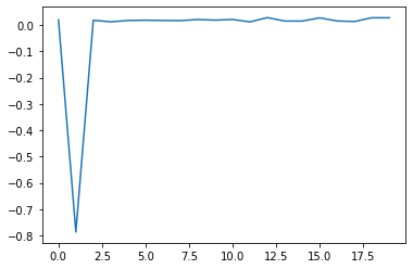
import matplotlib.pyplot as plt
plt.plot(list(range(len(history))), [a - 0.9 for a in history])
plt.show()

# It turns out that SGD with the given learning rate doesn't work well.
See also: